iLQR inference: reconstructing a zebrafish tail bout

A larval zebrafish swims in short bouts of tail undulation. Here a recurrent generative model of tail kinematics, trained as an iLQR-VAE, explains one recorded bout as the response of a latent dynamical system to a sparse sequence of inputs. Given the trained model, finding the most likely inputs for a new bout is a non-linear optimal control problem, which diffilqrax.ilqr.ilqr_solver solves.

Generative model. Latents \(x_t \in \mathbb{R}^{120}\) evolve under minimal gated unit (MGU2) dynamics driven by inputs \(u_t \in \mathbb{R}^{10}\), and are read out linearly into 7 tail-shape channels,

\[x_{t+1} = F(x_t, u_t), \qquad o_t \sim \mathcal{N}(c\,x_t + b,\ \mathrm{diag}(\sigma_o^2)), \qquad u_t \sim \text{Student-}t_\nu(0, \sigma_u).\]

The heavy-tailed Student-\(t\) prior favours inputs that are mostly small with occasional large kicks. The inferred inputs are the maximiser of \(\log p(u) + \log p(o \mid u)\), so the iLQR cost is the negative log joint: the prior on \(u_t\) plus the likelihood of the observation read out from \(x_t\).

The trained parameters and six bouts, with the inputs found by the original OCaml implementation, are stored in tests/fixtures/ocaml_mgu.npz, where the parity tests also use them.

from pathlib import Path
from typing import NamedTuple

import jax
import jax.numpy as jnp
import matplotlib.pyplot as plt
import numpy as onp
from jax.scipy.special import gammaln

from diffilqrax.ilqr import ilqr_solver, ilqr_simulate
from diffilqrax.typs import ModelDims, System, iLQRParams

jax.config.update("jax_enable_x64", True)

Data

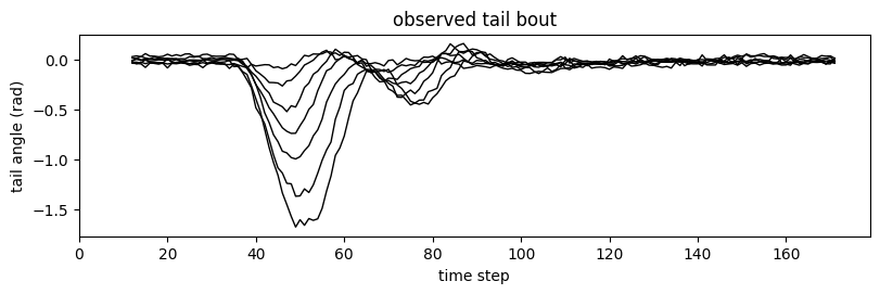
Each bout has \(T = 171\) steps. The first \(n_\text{beg} = 12\) steps only set the initial condition of the latents; the tail is observed for the remaining 160 steps. We take the last bout of the fixture.

data = dict(onp.load(Path("../../../tests/fixtures/ocaml_mgu.npz")))
p = {k[len("param_"):]: data[k] for k in data if k.startswith("param_")}
TRIAL, N_BEG = 5, 12
obs = data["saved_tail"][TRIAL]  # (160, 7) observed tail
T, m = data["ilqr_u"].shape[1:]
n, n_out = p["uh"].shape[0], p["c"].shape[0]
print(f"T={T}, latents n={n}, inputs m={m}, tail channels={n_out}")

t_obs = onp.arange(obs.shape[0]) + N_BEG
fig, ax = plt.subplots(figsize=(8, 2.6), layout="constrained")
# ax.plot(t_obs, obs + 2.0 * onp.arange(n_out), c="k", lw=1)

_ = ax.plot(t_obs, obs, c="k", lw=1)
_ = ax.set(xlabel="time step", ylabel="tail angle (rad)", title="observed tail bout", xlim=[0,None])

T=171, latents n=120, inputs m=10, tail channels=7

Defining the model

All parameters go into theta, a NamedTuple pytree. For \(t < n_\text{beg}\) the dynamics load the inputs into disjoint blocks of the latent state, \(x_{t+1} = x_t + B^{(t)\top} u_t\). Afterwards the MGU2 update is

\[f = \sigma(b_f + U_f^\top x), \qquad h = \tanh\!\big(b_h + U_h^\top (x \odot f)\big) + B^\top u, \qquad x' = (1 - f) \odot x + f \odot h .\]

class Theta(NamedTuple):
    B: jnp.ndarray  # (m, n) normalised input weights
    uh: jnp.ndarray  # (n, n)
    uf: jnp.ndarray  # (n, n)
    bh: jnp.ndarray  # (n,)
    bf: jnp.ndarray  # (n,)
    beg_bs: jnp.ndarray  # (n_beg, m, n) initial-condition loadings
    c: jnp.ndarray  # (n_out, n)
    bias: jnp.ndarray  # (n_out,)
    variances: jnp.ndarray  # (n_out,)
    sigma: jnp.ndarray  # (m,) Student-t scale
    sigma0: jnp.ndarray  # (m,) Gaussian scale of the first n_beg inputs
    nu: jnp.ndarray  # () degrees of freedom
    obs: jnp.ndarray  # (T - n_beg + 1, n_out)


k, i, j = onp.meshgrid(onp.arange(N_BEG), onp.arange(m), onp.arange(n), indexing="ij")
theta = Theta(
    B=jnp.sqrt(n / m) * p["wh"] / jnp.linalg.norm(p["wh"], axis=1, keepdims=True),
    uh=jnp.asarray(p["uh"]),
    uf=jnp.asarray(p["uf"]),
    bh=jnp.asarray(p["bh"]),
    bf=jnp.asarray(p["bf"]),
    beg_bs=jnp.asarray(((j // N_BEG == k) & (j % m == i)).astype(float)),
    c=jnp.asarray(p["c"]),
    bias=jnp.asarray(p["bias"]),
    variances=jnp.asarray(p["variances"]),
    sigma=jnp.sqrt((p["nu"] - 2.0) / p["nu"]) * p["spatial_stds"],
    sigma0=jnp.asarray(p["first_step"]),
    nu=jnp.asarray(p["nu"]),
    obs=jnp.asarray(obs),
)


def dynamics(t, x, u, theta):
    def load(_):
        return x + theta.beg_bs[jnp.minimum(t, N_BEG - 1)].T @ u

    def mgu(_):
        f = jax.nn.sigmoid(theta.bf + theta.uf.T @ x)
        h = jnp.tanh(theta.bh + theta.uh.T @ (x * f)) + theta.B.T @ u
        return (1.0 - f) * x + f * h

    return jax.lax.cond(t < N_BEG, load, mgu, None)


def readout(xs, theta):
    return theta.bias + xs @ theta.c.T

The cost: a sparse prior plus the likelihood

The running cost is the negative log prior of \(u_t\), Gaussian for the initial-condition steps and multivariate Student-\(t\) afterwards, plus the Gaussian negative log likelihood of observation \(t - n_\text{beg}\) given \(x_t\). There is no terminal cost. The Student-\(t\) term is not convex in \(u\), so the problem has local optima; iLQR uses its exact Hessian with Levenberg–Marquardt regularisation.

def prior(t, u, theta):
    gauss = 0.5 * (m * jnp.log(2 * jnp.pi) + 2 * jnp.sum(jnp.log(theta.sigma0)) + jnp.sum((u / theta.sigma0) ** 2))
    nu = theta.nu
    cst = gammaln(0.5 * nu) - gammaln(0.5 * (nu + m)) + 0.5 * m * jnp.log(jnp.pi * nu) + jnp.sum(jnp.log(theta.sigma))
    student = cst + 0.5 * (nu + m) * jnp.log1p(jnp.sum((u / theta.sigma) ** 2) / nu)
    return jnp.where(t < N_BEG, gauss, student)


def likelihood(t, x, theta):
    r = theta.obs[jnp.clip(t - N_BEG, 0, theta.obs.shape[0] - 1)] - (theta.bias + theta.c @ x)
    nll = 0.5 * (n_out * jnp.log(2 * jnp.pi) + jnp.sum(jnp.log(theta.variances)) + jnp.sum(r**2 / theta.variances))
    return jnp.where(t < N_BEG, 0.0, nll)


def cost(t, x, u, theta):
    return prior(t, u, theta) + likelihood(t, x, theta)


def costf(x, theta):
    return jnp.zeros(())


model = System(cost, costf, dynamics, ModelDims(n=n, m=m, horizon=T, dt=1.0))
params = iLQRParams(x0=jnp.zeros(n), theta=theta)

Solving

Starting from zero inputs, the solver runs until the KKT residual falls below kkt_tol. A first trial step of \(\alpha = 1\) (alpha_init=2.0) suits this problem better than the cautious default.

Us_zero = jnp.zeros((T, m))
solve = jax.jit(lambda u0: ilqr_solver(model, params, u0, max_iter=1000, alpha_init=2.0, kkt_tol=1e-6))
(Xs, Us, _), J_opt, cost_log = solve(Us_zero)
(X_zero, _), J_zero = ilqr_simulate(model, Us_zero, params)

J_ocaml = data["ilqr_cost"][TRIAL]
print(f"cost: {float(J_zero):.1f} (zero input) -> {float(J_opt):.3f} (diffilqrax), OCaml {J_ocaml:.3f}")
print(f"max |u* - u*_OCaml| = {float(jnp.abs(Us - data['ilqr_u'][TRIAL]).max()):.1e}")

cost: 23917.4 (zero input) -> -10403.917 (diffilqrax), OCaml -10403.917
max |u* - u*_OCaml| = 3.1e-07

For this bout both implementations reach the same optimum. On other bouts they can stop in different local optima of the non-convex objective, with costs that agree to about \(10^{-3}\).

Reconstruction

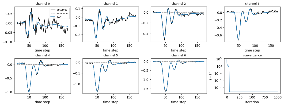
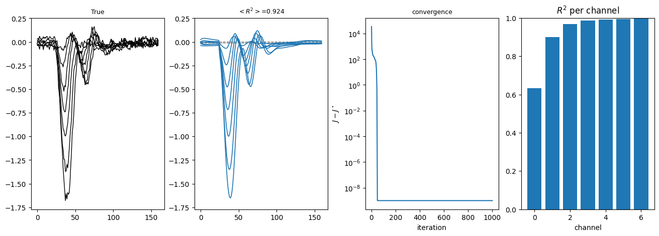
With zero input the latents relax to a fixed point and the readout is flat; the inferred inputs reproduce the bout. The latents saved by the solver are \(x_0 \dots x_T\), so observation \(j\) is read out from Xs[j + N_BEG].

o_zero = readout(X_zero[N_BEG:N_BEG + obs.shape[0]], theta)
o_opt = readout(Xs[N_BEG:N_BEG + obs.shape[0]], theta)
r2 = 1 - jnp.sum((o_opt - obs) ** 2) / jnp.sum((obs - obs.mean(0)) ** 2)
print(f"R^2 of the reconstruction: {float(r2):.3f}")

fig, axes = plt.subplots(2, 4, figsize=(12, 4.4), layout="constrained")
for ch, ax in enumerate(axes.flat[:n_out]):
    ax.plot(t_obs, obs[:, ch], c="k", lw=1, label="observed")
    ax.plot(t_obs, o_zero[:, ch], c="0.6", ls="--", lw=1, label="zero input")
    ax.plot(t_obs, o_opt[:, ch], c="C0", lw=1.2, label="iLQR")
    ax.set_title(f"channel {ch}", fontsize=9)
    ax.set_xlabel("time step")
axes.flat[0].legend(fontsize=7)
ax = axes.flat[-1]
ax.semilogy(cost_log - cost_log.min() + 1e-9, c="C0")
ax.set(xlabel="iteration", ylabel=r"$J - J^\star$", title="convergence")
ax.title.set_fontsize(9);

R^2 of the reconstruction: 0.993

# o_opt = onp.asarray(readout(theta, Xs))[N_BEG - 1 :]
# o_zero = onp.asarray(readout(theta, X_zero))[N_BEG - 1 :]
r2 = 1 - ((o_opt - obs) ** 2).sum(0) / ((obs - obs.mean(0)) ** 2).sum(0)

fig, axes = plt.subplots(1, 4, figsize=(13, 4.6), layout="constrained")
axes[0].plot(obs[:, :], c="k", lw=1, label="observed")
axes[0].set_title(f"True", fontsize=9)
axes[1].plot(o_zero[:, :], c="0.6", ls="--", lw=1, label="zero input")
axes[1].plot(o_opt[:, :], c="C0", lw=1.2, label="iLQR")
axes[1].set_title(f"$<R^2>$={r2.mean(0):.3f}", fontsize=9)

axes.flat[-1].bar(range(n_out), r2)
axes.flat[-1].set(ylim=(0, 1), xlabel="channel", title="$R^2$ per channel");

axes[0].sharey(axes[1])
ax = axes.flat[2]
ax.semilogy(cost_log - cost_log.min() + 1e-9, c="C0")
ax.set(xlabel="iteration", ylabel=r"$J - J^\star$", title="convergence")
ax.title.set_fontsize(9);

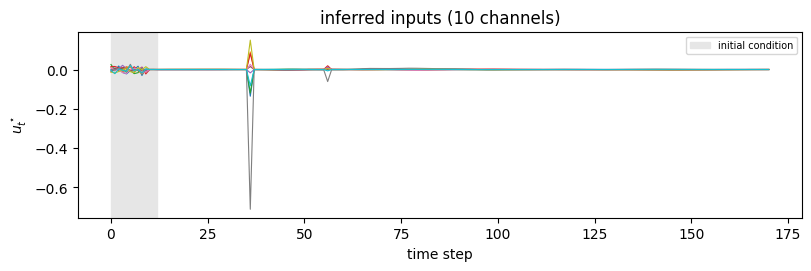
The inferred inputs are sparse, as the Student-\(t\) prior intends: one large kick that launches the bout, a smaller one a few beats later, and near-zero inputs elsewhere. The latent dynamics generate the undulation on their own.

fig, ax = plt.subplots(figsize=(8, 2.6), layout="constrained")
ax.plot(Us, lw=0.8)
ax.axvspan(0, N_BEG, color="0.9", label="initial condition")
ax.set(xlabel="time step", ylabel=r"$u^\star_t$", title="inferred inputs (10 channels)")
ax.legend(fontsize=7);

How to adapt

• Another bout: change TRIAL; only theta.obs depends on the bout, so solve is reused without recompiling.

• Many bouts at once: solve them as one batch with diffilqrax.batch, as in the next section; see batched iLQR for strategies and timings.

• Learning the model: the solution is differentiable with respect to theta (see gradients through iLQR), which is how an iLQR-VAE is trained.

• A Gaussian prior makes the cost convex in \(u\) for fixed latents and typically converges in fewer iterations, at the price of less sparse inputs.

Extension: many bouts at once

Only theta.obs changes from bout to bout, so all six bouts in the fixture can be solved as one batch inside one compiled program. batch.batched_ilqr_solver takes the batch axes as in jax.vmap: 0 for the batched leaf theta.obs, None for the shared ones. Its default strategy is jax.vmap.

The solver’s iterations, regularisation retries and line search are lax.while_loops, so under vmap the batch stops as soon as its slowest bout has converged. Bouts that finish early wait for it. On CPU, strategy="map" solves the bouts one after another instead; with several devices, strategy="shard" splits the batch across them. The batched iLQR notebook compares the strategies.

from diffilqrax import batch

all_obs = jnp.asarray(data["saved_tail"])  # (6, 160, 7)
obs_axes = iLQRParams(x0=None, theta=jax.tree.map(lambda _: None, theta)._replace(obs=0))
solve_all = jax.jit(
    lambda obs_batch: batch.batched_ilqr_solver(
        model, params._replace(theta=theta._replace(obs=obs_batch)), Us_zero, (obs_axes, None),
        max_iter=1000, alpha_init=2.0, kkt_tol=1e-6,
    )
)
(Xs_all, Us_all, _), J_all, log_all = solve_all(all_obs)

o_all = jax.vmap(lambda xs: readout(xs[N_BEG:N_BEG + all_obs.shape[1]], theta))(Xs_all)
r2_all = 1 - jnp.sum((o_all - all_obs) ** 2, axis=(1, 2)) / jnp.sum((all_obs - all_obs.mean(1, keepdims=True)) ** 2, axis=(1, 2))
log_all = onp.asarray(log_all)
# once converged the cost history repeats the final cost
iters = [int(onp.nonzero(h != h[-1])[0].max(initial=-1)) + 1 for h in log_all]

print(f"{'bout':>14s} {'J OCaml':>11s} {'J diffilqrax':>12s} {'rel diff':>9s} {'R^2':>6s} {'iters':>5s}")
for b in range(all_obs.shape[0]):
    J_oc = data["ilqr_cost"][b]
    label = f"{data['source'][b]}[{b}]"
    print(f"{label:>14s} {J_oc:11.3f} {float(J_all[b]):12.3f} {(float(J_all[b]) - J_oc) / abs(J_oc):9.1e} "
          f"{float(r2_all[b]):6.3f} {iters[b]:5d}")

          bout     J OCaml J diffilqrax  rel diff    R^2 iters
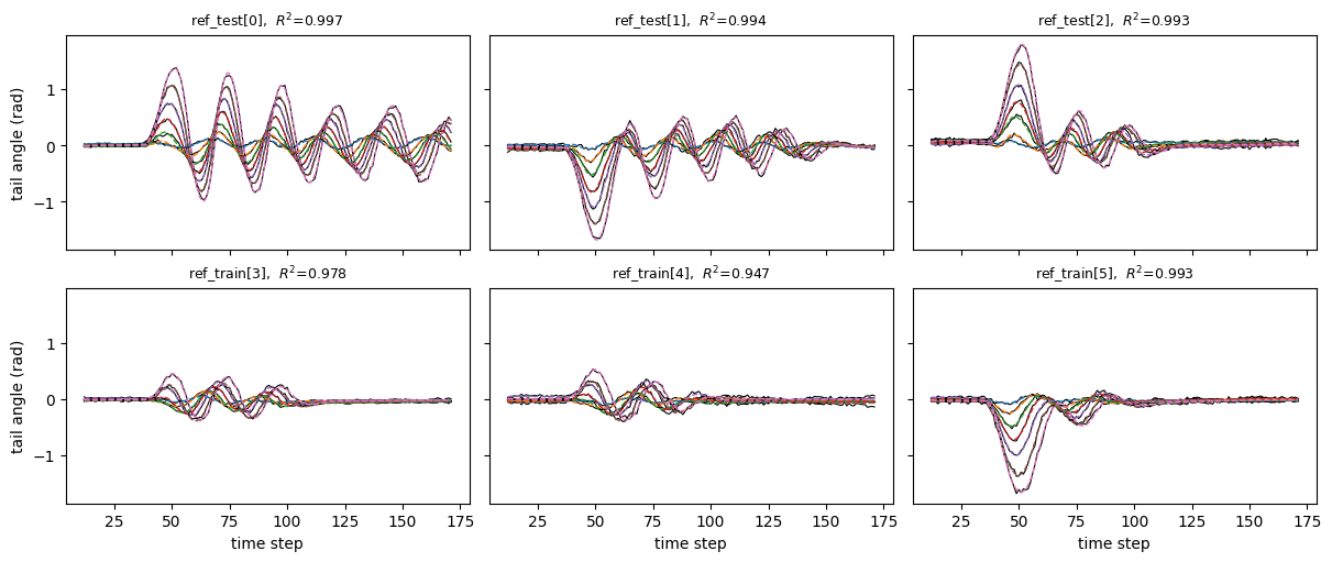
   ref_test[0]  -10215.129   -10188.690   2.6e-03  0.997    54
   ref_test[1]  -10297.255   -10302.552  -5.1e-04  0.994    51
   ref_test[2]  -10270.089   -10263.757   6.2e-04  0.993    77
  ref_train[3]  -10545.906   -10544.964   8.9e-05  0.978    40
  ref_train[4]  -10312.940   -10313.109  -1.6e-05  0.947    40
  ref_train[5]  -10403.917   -10403.917  -9.0e-14  0.993    53

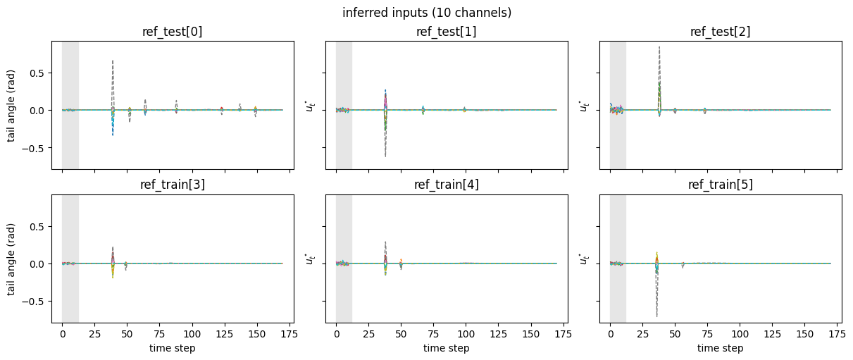
Bouts where the relative cost difference is not zero stopped in a different local optimum from OCaml, as noted above. Each panel overlays the seven observed channels (black) with their reconstruction (colour).

fig, axes = plt.subplots(2, 3, figsize=(12, 5), sharex=True, sharey=True, layout="constrained")
for b, ax in enumerate(axes.flat):
    ax.plot(t_obs, all_obs[b], c="k", lw=0.8)
    for ch in range(n_out):
        ax.plot(t_obs, o_all[b, :, ch], c=f"C{ch}", lw=1, ls="--")
    ax.set_title(f"{data['source'][b]}[{b}],  $R^2$={float(r2_all[b]):.3f}", fontsize=9)
for ax in axes[-1]:
    ax.set_xlabel("time step")
for ax in axes[:, 0]:
    ax.set_ylabel("tail angle (rad)")

fig, axes = plt.subplots(2, 3, figsize=(12, 5), sharex=True, sharey=True, layout="constrained")
for b, ax in enumerate(axes.flat):
    for ch in range(m):
        ax.plot(Us_all[b, :, ch], c=f"C{ch}", lw=1, ls="--")
    ax.set_title(f"{data['source'][b]}[{b}],  $R^2$={float(r2_all[b]):.3f}", fontsize=9)
    ax.set(
        ylabel=r"$u^\star_t$",
        title=f"{data['source'][b]}[{b}]",
    )
    ax.axvspan(0, N_BEG, color="0.9", label="initial condition")
for ax in axes[-1]:
    ax.set_xlabel("time step")
for ax in axes[:, 0]:
    ax.set_ylabel("tail angle (rad)")
fig.suptitle("inferred inputs (10 channels)")

Text(0.5, 0.98, 'inferred inputs (10 channels)')