

iLQR: swinging up a torque-limited pendulum#
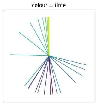
This notebook solves a non-linear optimal control problem with the iterative LQR solver diffilqrax.ilqr.ilqr_solver. A pendulum starts hanging down and must be swung up to the upright position within \(T\,\delta t = 5\) s. The motor cannot lift it directly, because the torque limit is smaller than \(mgl\), so the solver has to discover a pumping strategy.
Dynamics. With angle \(\phi\) measured from hanging down,
discretised with an Euler step. The state is \(x = (\phi, \dot\phi)\).
Cost. There is a small running cost on being away from upright, on velocity and on torque, plus a smooth barrier that keeps \(|u| \lesssim u_{\max}\). A large terminal cost asks for upright (\(\phi = \pm\pi\)) and still.
How iLQR works. Each iteration takes the current trajectory \((\bar x, \bar u)\) and forms a local LQR problem from first-order dynamics and second-order cost expansions. These are computed with jax.jacfwd/jax.hessian, so no hand-written derivatives are needed. The solver then:
solves the local LQR with a Riccati backward pass, adding Levenberg–Marquardt regularisation to the input Hessian until it is positive definite;
rolls out the non-linear dynamics under the new feedback policy \(u_t = \bar u_t + \alpha k_t + K_t(x_t - \bar x_t)\), choosing \(\alpha\) with an Armijo line search.
It stops when the input gradient of the Lagrangian \(\max_t|\partial L/\partial u_t|\) falls below kkt_tol.
[1]:
import jax
import jax.numpy as jnp
import jax.random as jr
import matplotlib.pyplot as plt

from diffilqrax.ilqr import ilqr_solver, ilqr_simulate, approx_lqr, kkt_input_residual
from diffilqrax.typs import System, ModelDims, iLQRParams, PendulumParams

jax.config.update("jax_enable_x64", True)
Defining the model#
A diffilqrax.typs.System bundles three functions and the problem dimensions:
cost(t, x, u, theta)is the running cost,costf(x, theta)is the terminal cost,dynamics(t, x, u, theta)returns \(x_{t+1}\).
theta can be any pytree of parameters. Here it is a PendulumParams(m, l, g). Keeping parameters in theta instead of hard-coding them is what makes them differentiable later (see gradients through iLQR).
[2]:
DT, DAMPING, U_MAX, HORIZON = 0.05, 0.1, 3.0, 100
dims = ModelDims(n=2, m=1, horizon=HORIZON, dt=DT)


def dynamics(t, x, u, theta):
    """Euler step; x = [angle, angular velocity], angle 0 is hanging down"""
    acc = -theta.g / theta.l * jnp.sin(x[0]) - DAMPING * x[1] + u[0] / (theta.m * theta.l**2)
    return x + DT * jnp.stack([x[1], acc])


def cost(t, x, u, theta):
    """Small running cost on angle, velocity and torque, plus a smooth barrier at |u| = U_MAX"""
    barrier = jax.nn.softplus(5.0 * (u - U_MAX)) ** 2 + jax.nn.softplus(5.0 * (-u - U_MAX)) ** 2
    return 0.1 * (1.0 + jnp.cos(x[0])) + 0.01 * x[1] ** 2 + 0.01 * jnp.sum(u**2) + jnp.sum(barrier)


def costf(x, theta):
    """Be upright (angle ±pi) and still at the final time"""
    return 50.0 * (1.0 + jnp.cos(x[0])) + 5.0 * x[1] ** 2


model = System(cost, costf, dynamics, dims)
params = iLQRParams(x0=jnp.array([0.1, 0.0]), theta=PendulumParams(m=1.0, l=1.0, g=9.8))
Us_init = 0.5 * jr.normal(jr.PRNGKey(0), (HORIZON, 1))
time = jnp.arange(HORIZON + 1) * DT
Solving#
The solver returns ((Xs, Us, lambdas), total_cost, cost_history). cost_history has length max_iter; after convergence its entries stay constant at the final cost.
[3]:
(Xs, Us, lambdas), total_cost, cost_log = ilqr_solver(model, params, Us_init, max_iter=300)

(X_init, _), J_init = ilqr_simulate(model, Us_init, params)
residual = kkt_input_residual(approx_lqr(model, Xs, Us, params))
print(f"cost: {float(J_init):.3f} (initial) -> {float(total_cost):.3f} (optimal)")
print(f"max|dL/du| = {jnp.max(jnp.abs(residual)):.1e}")
print(f"final angle {float(Xs[-1, 0]):.3f} rad (upright = ±{jnp.pi:.3f}), max|u| = {float(jnp.abs(Us).max()):.2f}")
cost: 118.408 (initial) -> 17.897 (optimal)
max|dL/du| = 8.7e-11
final angle -3.140 rad (upright = ±3.142), max|u| = 2.52
[4]:
fig, axes = plt.subplots(1, 3, figsize=(12, 3.2), layout="constrained")
axes[0].plot(time, X_init[:, 0], c="0.6", label="initial")
axes[0].plot(time, Xs[:, 0], c="C0", label="iLQR")
for s in (-1, 1):
    axes[0].axhline(s * jnp.pi, ls=":", c="k")
axes[0].set(xlabel="time (s)", ylabel="angle (rad)")
axes[0].legend()
axes[1].plot(time[:-1], Us[:, 0], c="C1")
for s in (-1, 1):
    axes[1].axhline(s * U_MAX, ls=":", c="k")
axes[1].set(xlabel="time (s)", ylabel="torque")
axes[2].semilogy(cost_log - cost_log.min() + 1e-12)
axes[2].set(xlabel="iteration", ylabel=r"$J - J^\star$");
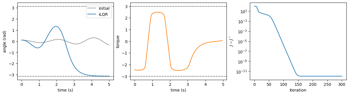
The torque limit is well below \(mgl\), so the solver discovers a pump: it swings one way, then the other, and finally over the top, all while staying within the limit. The cost drops by most of its initial value within the first ~20 iterations. After that the solver converges linearly down to the round-off level of the cost. The default first trial step is \(\alpha = \tau \cdot \texttt{alpha\_init} = 0.5\), which is cautious but robust.
[5]:
fig, ax = plt.subplots(figsize=(4, 4))
for i in range(0, HORIZON + 1, 4):
    px, py = jnp.sin(Xs[i, 0]), -jnp.cos(Xs[i, 0])
    ax.plot([0, px], [0, py], c=plt.cm.viridis(i / HORIZON), alpha=0.8)
ax.set(aspect="equal", xlim=(-1.2, 1.2), ylim=(-1.2, 1.2), xticks=[], yticks=[], title="colour = time");
How to adapt#
Your own system: replace
dynamicswith any differentiable JAX function of(t, x, u, theta)and updateModelDims(n, m, horizon, dt). For stiff or fast dynamics, use a better integrator (for example RK4) insidedynamics.Costs: any twice-differentiable scalar function works. Use smooth penalties (softplus, as here) for limits, because hard
clip/maxhave zero curvature and slow iLQR down.Initial guess: iLQR is a local method. A non-zero
Us_init(here a little noise) can break symmetries, and a feasible heuristic speeds up hard problems.Convergence:
kkt_tol(default1e-10) sets the stopping test andmax_itercaps the iterations. Line-search options (tau,beta,alpha_min,max_iter_linesearch) are passed through as keyword arguments.alpha_init=2.0makes the first trial a full Newton step (\(\alpha = 1\)).Compile once, solve many: wrap the call in
jax.jit(withmodelclosed over) when solving repeatedly, for example in MPC or in a training loop.