

Implicit gradients through the iLQR solver#
Often the optimal trajectory is just one component of a larger model. Examples are learning the dynamics or cost parameters \(\theta\) from data (inverse optimal control), or using a planner as a layer in a neural network, as in iLQR-VAE [Schimel et al., 2022]. Training such a model needs \(\partial \tau^\star(\theta) / \partial\theta\), where \(\tau^\star = (x^\star, u^\star)\) is the solution.
There are two ways to get these gradients:
Direct: backpropagate through every iteration of the solver. This is exact for the unrolled computation, but memory grows with the number of iterations, and the gradient depends on the solver’s path as well as its solution.
Implicit: differentiate the optimality (KKT) conditions at the solution, as OptNet [Amos and Kolter, 2017] does for quadratic programs. By the implicit function theorem, the vector–Jacobian product is the solution of another LQR problem built from the Hessian of the Lagrangian. Its cost is about one extra LQR solve, independent of the number of solver iterations.
diffilqrax.diff_ilqr.dilqr implements the implicit approach as a jax.custom_vjp. It returns \(\tau^\star = [x_t, u_t]\), an array of shape (T+1, n+m) whose last row of \(u\) is padded with zeros. You can call jax.grad on it like any other JAX function.
[1]:
import jax
import jax.numpy as jnp
import jax.random as jr
import matplotlib.pyplot as plt

from diffilqrax.diff_ilqr import dilqr
from diffilqrax.ilqr import ilqr_solver
from diffilqrax.typs import System, ModelDims, iLQRParams, Theta

jax.config.update("jax_enable_x64", True)
The problem#
A small recurrent network \(x_{t+1} = U_h \tanh(x_t) + W_h \tanh(u_t)\) must track a sine target under a learnable state cost \(Q\). The parameters are \(\theta = (U_h, W_h, Q)\).
[2]:
dims = ModelDims(n=6, m=2, horizon=60, dt=0.1)
k1, k2, k3 = jr.split(jr.PRNGKey(0), 3)
L = 0.5 * jr.normal(k3, (dims.n, dims.n)) / jnp.sqrt(dims.n)
theta = Theta(
    Uh=0.5 * jr.normal(k1, (dims.n, dims.n)) / jnp.sqrt(dims.n),
    Wh=0.5 * jr.normal(k2, (dims.n, dims.m)) / jnp.sqrt(dims.n),
    sigma=jnp.zeros(dims.n),
    Q=L @ L.T + 0.1 * jnp.eye(dims.n),
)
params = iLQRParams(x0=jnp.zeros(dims.n), theta=theta)


def cost(t, x, u, theta):
    err = x - jnp.sin(t / 5.0)
    return err @ theta.Q @ err + jnp.sum(u**2)


def costf(x, theta):
    return jnp.sum(x**2)


def dynamics(t, x, u, theta):
    return theta.Uh @ jnp.tanh(x) + theta.Wh @ jnp.tanh(u)


model = System(cost, costf, dynamics, dims)
Us_init = jnp.zeros((dims.horizon, dims.m))
solver_kwargs = dict(max_iter=100, kkt_tol=1e-10)
A loss on the optimal trajectory#
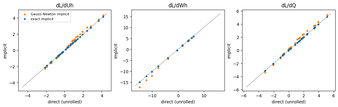
As an example outer objective, take the squared norm of the optimal trajectory, \(\mathcal{L}(\theta) = \lVert x^\star(\theta)\rVert^2 + \lVert u^\star(\theta)\rVert^2\). We compare three gradients:
implicit:
dilqrwith the exact Lagrangian Hessian (the default,exact_hessian=True);direct:
jax.gradthrough every iteration ofilqr_solver;Gauss–Newton implicit:
dilqr(..., exact_hessian=False), which drops the dynamics curvature \(\lambda^\top \nabla^2 f\). It is cheaper, but exact only for linear dynamics.
[3]:
def implicit_loss(theta, exact_hessian=True):
    tau = dilqr(model, iLQRParams(params.x0, theta), Us_init, exact_hessian=exact_hessian, **solver_kwargs)
    return jnp.sum(tau**2)


def direct_loss(theta):
    (Xs, Us, _), _, _ = ilqr_solver(model, iLQRParams(params.x0, theta), Us_init, **solver_kwargs)
    return jnp.sum(Xs**2) + jnp.sum(Us**2)


val_imp, g_imp = jax.value_and_grad(implicit_loss)(theta)
val_dir, g_dir = jax.value_and_grad(direct_loss)(theta)
g_gn = jax.grad(lambda th: implicit_loss(th, exact_hessian=False))(theta)
print(f"loss: implicit {float(val_imp):.8f}, direct {float(val_dir):.8f}")
loss: implicit 4.68615848, direct 4.68615848
[4]:
names = ["Uh", "Wh", "Q"]
fig, axes = plt.subplots(1, 3, figsize=(11, 3.4), layout="constrained")
for ax, name in zip(axes, names):
    d = getattr(g_dir, name).ravel()
    ax.scatter(d, getattr(g_gn, name).ravel(), s=12, c="C1", label="Gauss–Newton implicit")
    ax.scatter(d, getattr(g_imp, name).ravel(), s=12, c="C0", label="exact implicit")
    lim = jnp.abs(d).max() * 1.1
    ax.plot([-lim, lim], [-lim, lim], "k:", lw=1)
    ax.set(title=f"dL/d{name}", xlabel="direct (unrolled)", ylabel="implicit")
axes[0].legend(fontsize=8);
[5]:
def rel_err(a, b):
    return float(jnp.linalg.norm(a - b) / jnp.linalg.norm(b))

for name in names:
    print(f"{name:3s} exact implicit vs direct: {rel_err(getattr(g_imp, name), getattr(g_dir, name)):.1e}   "
          f"Gauss–Newton vs direct: {rel_err(getattr(g_gn, name), getattr(g_dir, name)):.1e}")
Uh  exact implicit vs direct: 1.0e-10   Gauss–Newton vs direct: 1.3e-01
Wh  exact implicit vs direct: 9.5e-11   Gauss–Newton vs direct: 1.4e-01
Q   exact implicit vs direct: 4.9e-11   Gauss–Newton vs direct: 1.4e-01
The exact implicit gradient matches backpropagation through the converged solver to about \(10^{-10}\) relative error, the level of the solver tolerance, without storing the solver’s iterations. The Gauss–Newton variant is visibly biased here because the dynamics are non-linear. For linear dynamics the two coincide.
How to adapt#
Learnable parameters: anything inside
params.theta(any pytree), andparams.x0, receives gradients. Put whatever you want to learn there and read it incost,costfanddynamics.Outer loss:
dilqrreturnstauof shape(T+1, n+m). Slicetau[:, :n]for states andtau[:-1, n:]for inputs, and build any differentiable loss on them, for example a fit to observed trajectories.Converge tightly: implicit gradients assume the KKT conditions hold, so keep
kkt_tolsmall (float64 is enabled by default).LQR problems: use
diffilqrax.diff_lqr.dlqrwithLQRParams. For long horizons on a GPU, use the parallel versionsdiffilqrax.parallel_dilqr.pdilqranddiffilqrax.parallel_dlqr.pdlqr.