LQR: bringing a double integrator to rest

This notebook solves a finite-horizon linear quadratic regulator (LQR) problem with diffilqrax.lqr.solve_lqr. It then checks the solution against the KKT optimality conditions and against the parallel solver diffilqrax.plqr.solve_plqr.

The problem. The state is a position and velocity, \(x = (p, v)\), and the input \(u\) is an acceleration. The discretised dynamics with time step \(\delta t\) are

\[\begin{split}x_{t+1} = A x_t + B u_t, \qquad A = \begin{pmatrix} 1 & \delta t \\ 0 & 1 \end{pmatrix}, \quad B = \begin{pmatrix} \tfrac12 \delta t^2 \\ \delta t \end{pmatrix}.\end{split}\]

We want to bring the state to rest at the origin using little control effort, so we minimise

\[J = \tfrac12 x_T^\top Q_f x_T + \sum_{t=0}^{T-1} \tfrac12 \left( x_t^\top Q x_t + u_t^\top R u_t \right).\]

from functools import partial

import jax
import jax.numpy as jnp
import jax.random as jr
import matplotlib.pyplot as plt

from diffilqrax.lqr import solve_lqr, kkt
from diffilqrax.plqr import solve_plqr
from diffilqrax.typs import LQR, LQRParams, ModelDims

jax.config.update("jax_enable_x64", True)

Setting up the problem

diffilqrax uses the general time-varying LQR cost

\[\ell_t(x, u) = \tfrac12 x^\top Q_t x + q_t^\top x + \tfrac12 u^\top R_t u + r_t^\top u + x^\top S_t u, \qquad x_{t+1} = A_t x_t + B_t u_t + a_t ,\]

with terminal cost \(\tfrac12 x^\top Q_f x + q_f^\top x\). Every time-varying term is stacked along a leading time axis of length \(T\). This problem is time-invariant, so we tile each matrix \(T\) times.

dims = ModelDims(n=2, m=1, horizon=100, dt=0.1)
T, n, m = dims.horizon, dims.n, dims.m

A = jnp.array([[1.0, dims.dt], [0.0, 1.0]])
B = jnp.array([[0.5 * dims.dt**2], [dims.dt]])

span_mat = partial(jnp.tile, reps=(T, 1, 1))  # (n, k) -> (T, n, k)
span_vec = partial(jnp.tile, reps=(T, 1))     # (n,)   -> (T, n)

lqr = LQR(
    A=span_mat(A),
    B=span_mat(B),
    a=span_vec(jnp.zeros(n)),
    Q=span_mat(jnp.eye(n)),
    q=span_vec(jnp.zeros(n)),
    R=span_mat(jnp.eye(m)),
    r=span_vec(jnp.zeros(m)),
    S=span_mat(jnp.zeros((n, m))),
    Qf=jnp.eye(n),
    qf=jnp.zeros(n),
)

x0 = jr.normal(jr.PRNGKey(0), (n,))
params = LQRParams(x0=x0, lqr=lqr)
print("initial state:", x0)

initial state: [ 1.81608667 -0.75488484]

Solving

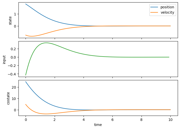
solve_lqr runs a Riccati backward pass and then a forward rollout. It returns the optimal states \(x_{0:T}\), the inputs \(u_{0:T-1}\) and the costates (Lagrange multipliers) \(\lambda_{0:T}\).

Xs, Us, lambdas = solve_lqr(params)
print(Xs.shape, Us.shape, lambdas.shape)

(101, 2) (100, 1) (101, 2)

time = jnp.arange(T + 1) * dims.dt
fig, axes = plt.subplots(3, 1, figsize=(7, 5), sharex=True, layout="constrained")
axes[0].plot(time, Xs, label=["position", "velocity"])
axes[0].legend()
axes[1].plot(time[:-1], Us, c="C2")
axes[2].plot(time, lambdas)
for ax, label in zip(axes, ["state", "input", "costate"]):
    ax.set_ylabel(label)
axes[-1].set_xlabel("time");

Checking optimality

At the optimum, the gradients of the Lagrangian with respect to \(x\), \(u\) and \(\lambda\) are zero. diffilqrax.lqr.kkt returns these residuals. They should be at the level of float64 round-off.

dLdX, dLdU, dLdLambda = kkt(params, Xs, Us, lambdas)
for name, r in [("dL/dx", dLdX), ("dL/du", dLdU), ("dL/dλ", dLdLambda)]:
    print(f"max|{name}| = {jnp.max(jnp.abs(r)):.2e}")

max|dL/dx| = 0.00e+00
max|dL/du| = 1.89e-15
max|dL/dλ| = 2.78e-17

The parallel solver uses an associative scan instead of the sequential recursion. It returns the same solution:

Xp, Up, _ = solve_plqr(params)
print(f"max|Xs - Xp| = {jnp.max(jnp.abs(Xs - Xp)):.2e},  max|Us - Up| = {jnp.max(jnp.abs(Us - Up)):.2e}")

max|Xs - Xp| = 4.44e-16,  max|Us - Up| = 1.28e-15

How to adapt

• Your own linear system: replace A, B and dims. If the system is time-varying, build arrays of shape (T, n, n) and (T, n, m) directly instead of tiling.

• Costs: a larger R relative to Q gives gentler inputs and slower convergence. Qf sets how strongly the final state is pinned. Q, Qf must be positive semi-definite and R positive definite.

• Offsets and cross terms: use a for affine dynamics (for example gravity) and S for state–input coupling in the cost.

• Tracking a target: use the linear terms q and qf, as shown in the tracking example.

• Long horizons on a GPU: switch to solve_plqr. It has the same inputs and outputs.