Parallel (associative-scan) solvers

The Riccati recursion in LQR is sequential: step \(t\) needs step \(t+1\). However, the recursion can be rewritten as an associative combination of per-step elements, which jax.lax.associative_scan evaluates in \(O(\log T)\) parallel depth (Särkkä & García-Fernández, 2023). diffilqrax provides parallel counterparts of every solver:

sequential	parallel
lqr.solve_lqr	plqr.solve_plqr
ilqr.ilqr_solver	parallel_ilqr.pilqr_solver
diff_lqr.dlqr	parallel_dlqr.pdlqr
diff_ilqr.dilqr	parallel_dilqr.pdilqr

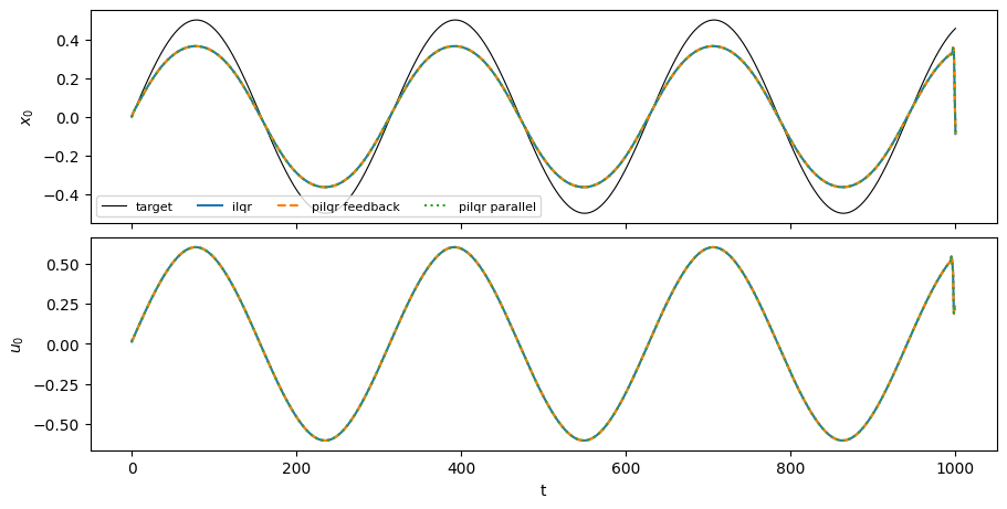
The parallel versions take the same arguments and converge to the same solutions. This notebook checks that on a long-horizon iLQR problem and shows how run time scales with the horizon.

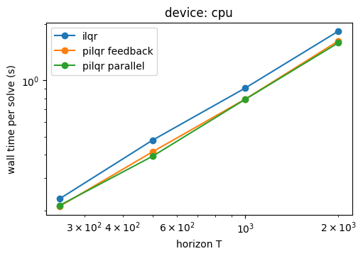
The parallel solvers do more total work, so on a CPU you should not expect a speed-up; at best they roughly match the sequential solver. The benefit appears on a GPU with long horizons, where the sequential solver is limited by its \(O(T)\) depth.

import time as timer

import jax
import jax.numpy as jnp
import jax.random as jr
import matplotlib.pyplot as plt

from diffilqrax.ilqr import ilqr_solver
from diffilqrax.parallel_ilqr import pilqr_solver, dynamics_defects
from diffilqrax.diff_ilqr import dilqr
from diffilqrax.parallel_dilqr import pdilqr
from diffilqrax.typs import System, ModelDims, iLQRParams, Theta

jax.config.update("jax_enable_x64", True)
print("device:", jax.devices()[0])

device: TFRT_CPU_0

A long-horizon problem

A stable tanh RNN, \(x_{t+1} = \tanh(U_h x_t + W_h u_t)\), tracks a slow sine wave in every state.

N, M = 8, 3
k1, k2 = jr.split(jr.PRNGKey(0))
theta = Theta(Uh=0.8 * jr.normal(k1, (N, N)) / jnp.sqrt(N), Wh=jr.normal(k2, (N, M)) / jnp.sqrt(N), sigma=0.0, Q=None)


def make_model(horizon):
    def cost(t, x, u, th):
        return jnp.sum((x - 0.5 * jnp.sin(t / 50.0)) ** 2) + 0.1 * jnp.sum(u**2)

    def costf(x, th):
        return jnp.sum(x**2)

    def dynamics(t, x, u, th):
        return jnp.tanh(th.Uh @ x + th.Wh @ u)

    return System(cost, costf, dynamics, ModelDims(n=N, m=M, horizon=horizon, dt=0.1))


params = iLQRParams(x0=jnp.zeros(N), theta=theta)

Same solution

pilqr_solver has two ways to roll out a candidate step:

• rollout="feedback" (default) runs the parallel Riccati scan, then a sequential non-linear rollout under the feedback policy, exactly like ilqr_solver. Every iterate is a feasible trajectory.

• rollout="parallel" uses multiple shooting. The states are also optimisation variables, the dynamics defects \(d_t = f(x_t, u_t) - x_{t+1}\) enter the local LQR, and the whole step is computed with associative scans. Iterates are feasible only at convergence, so we report the largest defect.

T = 1000
model = make_model(T)
Us_init = jnp.zeros((T, M))

(Xs, Us, _), J, _ = ilqr_solver(model, params, Us_init, max_iter=200)
(Xf, Uf, _), Jf, _ = pilqr_solver(model, params, Us_init, max_iter=200, rollout="feedback")
(Xp, Up, _), Jp, _ = pilqr_solver(model, params, Us_init, max_iter=200, rollout="parallel")

print(f"ilqr             J = {float(J):.10f}")
print(f"pilqr feedback   J = {float(Jf):.10f}   max|ΔU| = {jnp.max(jnp.abs(Uf - Us)):.1e}")
print(f"pilqr parallel   J = {float(Jp):.10f}   max|ΔU| = {jnp.max(jnp.abs(Up - Us)):.1e}   "
      f"max defect = {jnp.max(jnp.abs(dynamics_defects(model, params, Xp, Up))):.1e}")

ilqr             J = 745.6031498673
pilqr feedback   J = 745.6031498673   max|ΔU| = 1.2e-15
pilqr parallel   J = 745.6031498673   max|ΔU| = 7.0e-13   max defect = 3.3e-16

time = jnp.arange(T + 1)
fig, axes = plt.subplots(2, 1, figsize=(9, 4.5), sharex=True, layout="constrained")
axes[0].plot(time, 0.5 * jnp.sin(time / 50.0), "k", lw=0.8, label="target")
for (X, U), style, label in [((Xs, Us), "-", "ilqr"), ((Xf, Uf), "--", "pilqr feedback"), ((Xp, Up), ":", "pilqr parallel")]:
    axes[0].plot(time, X[:, 0], style, label=label)
    axes[1].plot(time[:-1], U[:, 0], style)
axes[0].set(ylabel="$x_0$")
axes[1].set(ylabel="$u_0$", xlabel="t")
axes[0].legend(ncol=4, fontsize=8);

Gradients agree too

pdilqr is the parallel counterpart of dilqr. Both the forward solve and the adjoint LQR in the reverse pass use associative scans.

Ts = 200
model_s = make_model(Ts)
U0 = jnp.zeros((Ts, M))


def loss(solver, th):
    return jnp.sum(solver(model_s, iLQRParams(params.x0, th), U0, max_iter=200) ** 2)


g_seq = jax.grad(lambda th: loss(dilqr, th))(theta)
g_par = jax.grad(lambda th: loss(pdilqr, th))(theta)
for name in ("Uh", "Wh"):
    a, b = getattr(g_par, name), getattr(g_seq, name)
    print(f"dL/d{name}: relative difference {jnp.linalg.norm(a - b) / jnp.linalg.norm(b):.1e}")

dL/dUh: relative difference 9.8e-15
dL/dWh: relative difference 7.1e-15

Scaling with the horizon

We time one jitted solve at several horizons. The absolute numbers depend on your hardware. On a CPU, all three scale linearly and take similar time. On a GPU, the "parallel" rollout should scale best.

def time_solver(solve, model, n_repeat=3):
    Us0 = jnp.zeros((model.dims.horizon, M))
    f = jax.jit(lambda p, u: solve(model, p, u, max_iter=200))
    jax.block_until_ready(f(params, Us0))  # compile
    start = timer.perf_counter()
    for _ in range(n_repeat):
        jax.block_until_ready(f(params, Us0))
    return (timer.perf_counter() - start) / n_repeat


solvers = {
    "ilqr": ilqr_solver,
    "pilqr feedback": lambda m, p, u, **kw: pilqr_solver(m, p, u, rollout="feedback", **kw),
    "pilqr parallel": lambda m, p, u, **kw: pilqr_solver(m, p, u, rollout="parallel", **kw),
}
horizons = [250, 500, 1000, 2000]
timings = {name: [time_solver(s, make_model(h)) for h in horizons] for name, s in solvers.items()}

fig, ax = plt.subplots(figsize=(5, 3.5), layout="constrained")
for name, ts in timings.items():
    ax.loglog(horizons, ts, "o-", label=name)
ax.set(xlabel="horizon T", ylabel="wall time per solve (s)", title=f"device: {jax.devices()[0].platform}")
ax.legend();

How to adapt

• Switching solver: replace ilqr_solver with pilqr_solver (or dilqr with pdilqr). The model, parameters and initial inputs are unchanged.

• Choosing a rollout: use "feedback" when you need every iterate to be feasible, for example when stopping early. Use "parallel" for the most parallelism on a GPU.

• Non-convex costs: make_psd="R" or "full" projects the local problem to be convex, which makes every scan element valid without regularisation retries.

• Gradient adjoint: pdilqr(..., adjoint="sequential") solves the reverse LQR sequentially. This is useful for checking results or on a CPU.

• Benchmarking on a GPU: install a CUDA build of JAX and re-run this notebook. For a script version, see examples/long_horizon.py in the repository.