Balanced Model Order Reduction Tutorial

Overview

Balanced model order reduction is a systematic approach to approximating high-dimensional dynamical systems with lower-dimensional models while preserving key system properties. This technique is particularly useful in control theory and computational modeling where computational efficiency is crucial.

Mathematical Foundation

Consider a linear time-invariant system:

ẋ = Ax + Bu\\
y = Cx + Du

Where:

• $x \in \mathbb{R}^{n}$ is the state vector
• $u \in \mathbb{R}^{m}$ is the input vector
• $y \in \mathbb{R}^{p}$ is the output vector
• $A$, $B$, $C$, $D$ are system matrices

Key Concepts

Controllability and Observability Gramians

The controllability Gramian $W_c$ measures how much energy is required to reach each state:

AW_c + W_cAᵀ + BBᵀ = 0

The observability Gramian $W_o$ measures how well each state can be observed from the output:

AᵀW_o + W_oA + CᵀC = 0

Hankel Singular Values

The Hankel singular values $\sigma_i$ where $i=(1,\dots,n)$ are the square roots of the eigenvalues of $W_c W_o$:

\sigma_i = \sqrt{\lambda_i(W_cW_o)}

These values indicate the “importance” of each state - larger values correspond to states that are both highly controllable and observable.

Balanced Realization Algorithm

1. Solve Lyapunov equations to find $W_c$ and $W_o$

2. Compute the Cholesky decomposition: $W_c = R R^{\text{T}}$

3. Perform SVD on $R^{\text{T}}W_o R = U\Sigma V^{\text{T}}$

4. Form transformation matrices:

   \begin{align*}
   T = R^{\text{-T}}U\Sigma^{-1/2} \\
   T^{\text{-1}} = \Sigma^{1/2}V^{\text{T}}R^{\text{T}}
   \end{align*}
   

5. Transform the system:

   \tilde{A} = T^{-1}AT, \;\;\; \tilde{B} = T^{-1}B, \;\;\; \tilde{C} = CT
   

Model Reduction

After balancing, truncate the system by keeping only the $r$ most significant states (largest Hankel singular values):

\begin{align*}
A^{(r)} &= \tilde{A}^{(r \times r)} \\
B^{(r)} &= \tilde{B}^{(r \times m)} \\
C^{(r)} &= \tilde{C}^{(p \times r)} \\
D^{(r)} &= D
\end{align*}

Error Bounds

The approximation error is bounded by:

||G - G_r||_{\infty} ≤ 2\sum_{i=r+1}^{n} σᵢ

Where $G$ and $G_r$ are the transfer functions of the original and reduced systems.

Advantages

• Preservation of stability: Balanced truncation preserves system stability
• Error bounds: Provides computable error bounds
• Systematic approach: No trial-and-error required
• Physical insight: Hankel singular values provide insight into system behavior

Applications

• Control system design: Reducing controller complexity
• Structural dynamics: Simplifying finite element models
• Circuit analysis: Reducing large-scale circuit models
• Fluid dynamics: Reducing CFD models for real-time applications

Python example

Here is a quick implementation of the steps above:

import numpy as np
import scipy.linalg as slinalg

# Step 1:
Q = B.dot(B.T)
W_c = slinalg.solve_discrete_lyapunov(A, Q, method="direct")

P = C.T.dot(C)
W_o = slinalg.solve_discrete_lyapunov(A, P, method="direct")

# Step 2:
R = slinalg.cholesky(W_c, lower=True)
R_h = R.T.conj()

# Step 3:
sig_sqr, U = slinalg.eig(R_h@W_o@R)
sig_sqr = sig_sqr.astype(complex)

# Step 4:
T_bal = np.diag(sig_sqr**0.25) @ U.T.conj() @ LA.inv(R)
T_inv_bal = R @ U @ np.diag(sig_sqr**-0.25)

# Step 5:
A_tilde = T_bal @ A @ T_inv_bal
B_tilde = T_bal @ B
C_tilde = C @ T_inv_bal

# Validation:
sig_Wc = np.diag(T_bal @ W_c @ T_bal.T.conj())
sig_Wo = np.diag(T_inv_bal.T.conj() @ W_o @ T_inv_bal)

print("Σ_c == Σ_o:", np.allclose(np.real(sig_Wc),np.real(sig_Wo)))

Test if the system is fully controllable and observable, a criteria essential for balanced model reduction:

def controlability(A:np.ndarray, B:np.ndarray)->Tuple[np.ndarray, int]:
   import numpy.linalg as linalg
    n = A.shape[0]
    ctrb = np.hstack(
            [B.T] + [LA.matrix_power(A, i) @ B.T
                    for i in range(1, n)])
    return ctrb, linalg.matrix_rank(ctrb)

def observability(A:np.ndarray, C:np.ndarray)->Tuple[np.ndarray, int]:
   import numpy.linalg as linalg
    n = A.shape[0]
    obsv = np.hstack(
            [C] + [LA.matrix_power(A, i) @ C
                    for i in range(1, n)])
    return obsv.T, linalg.matrix_rank(obsv)

Application: Reduced model of C. Elegans locomotion

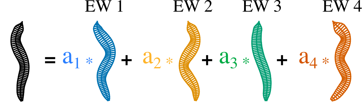
The posture of the worm can be captured by 4 principal components (aka eigen-worms)

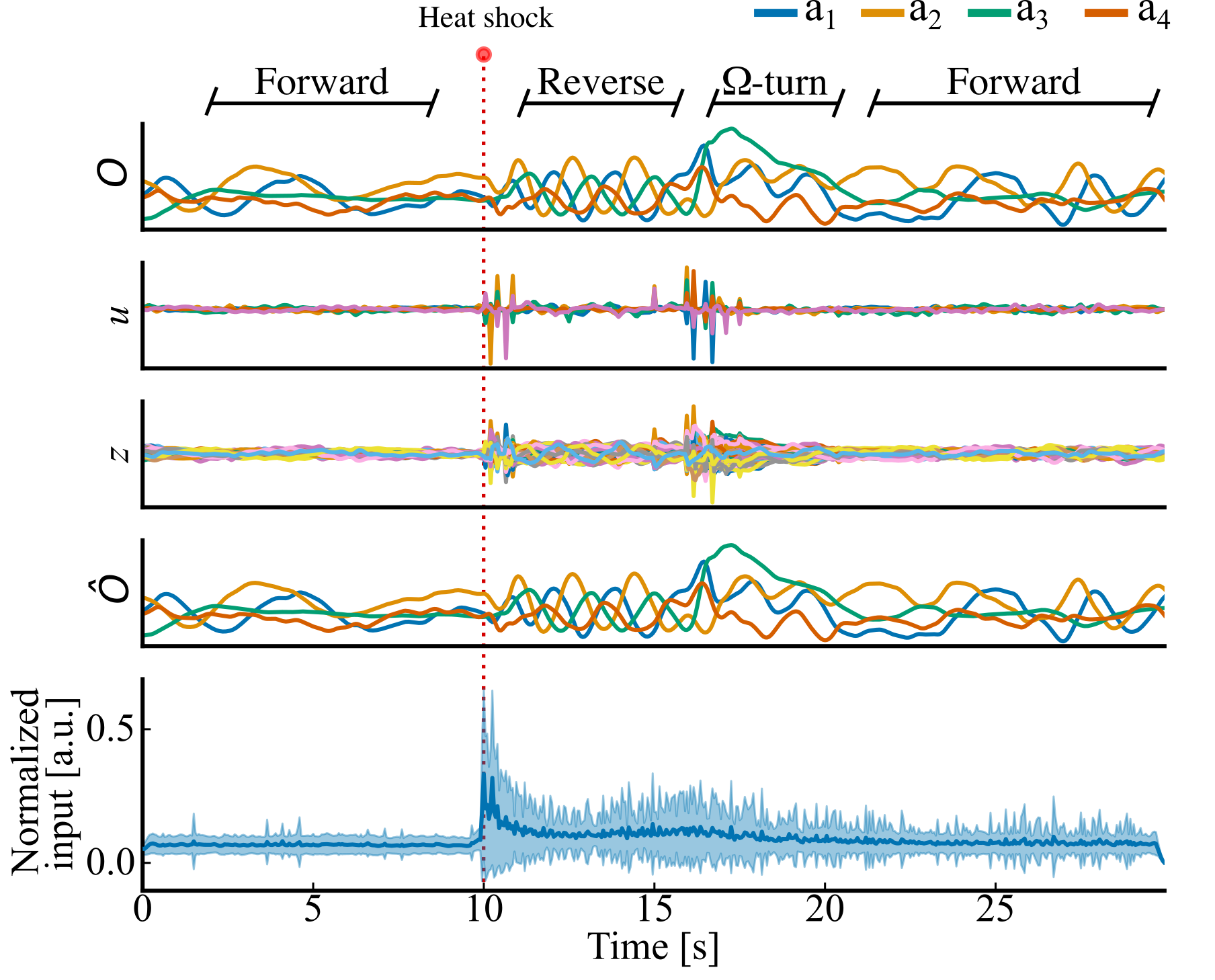
We trained a 60 dimensional linear network with 5 inputs to capture the postural dynamics of the worm.

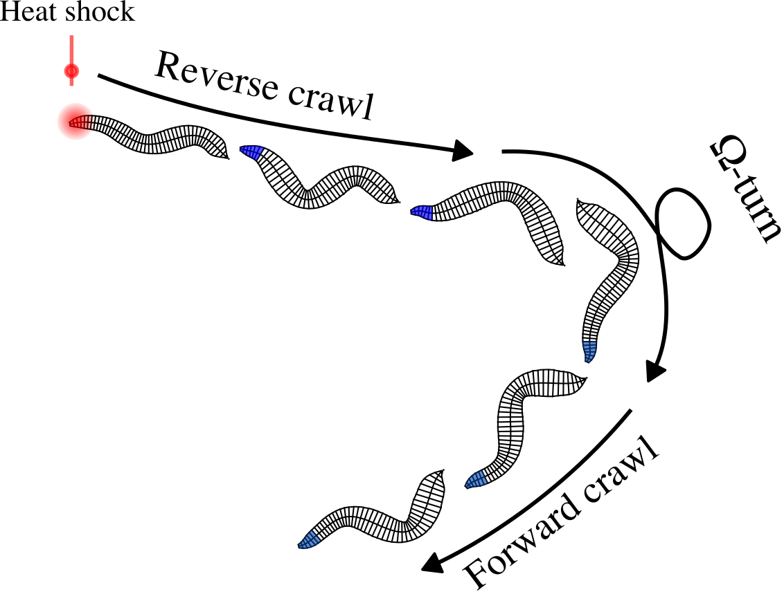
The trained model could infer control to capture the characteristic escape sequence of worm (reverse crawl $\rightarrow$ high-angle Ω-turn $\rightarrow$ forward crawl)

The first four plots are an example trial (True PC trajectories, inferred control inputs to the RNN, 60 unit RNN activity, Reconstructed PC trajectories). The red line indicated the aversive stimulus, triggering the escape sequence. The bottom plot shows the inferred control for all trials aligned on the external stimulus.

We used Balanced Model Reduction to compress the learned RNN dynamics to 20 dimensions and interpret the underlying dynamics.

The three slowest decaying eigenmodes of the reduced model mapped to reverse crawl, Ω-turn, and forward crawl behavioral states.

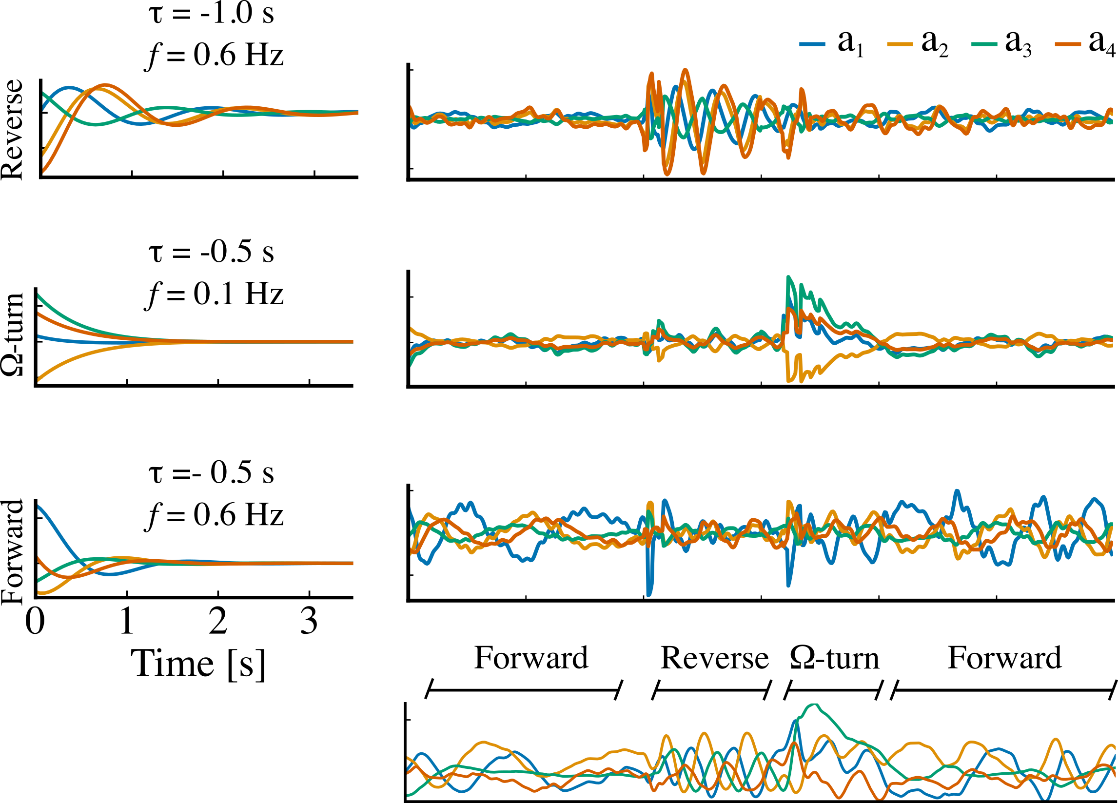
Details can be found in this paper.

Conclusion

Balanced model order reduction provides a principled way to reduce system complexity while maintaining essential dynamics. The method’s theoretical guarantees and practical effectiveness make it a cornerstone technique in modern control theory and computational modeling.