Probabilistic Spiking Model
Published:
My summer project involved fitting a generalised linear model (GLM) to generated spiking data. I aimed to learn how to fit a GLM to data from scratch and understand how it can be used to simulate and predict spiking activity in response to external inputs corresponding to sensory stimuli. In this article, I will outline the theory behind GLMs and demonstrate the results of applying this method to simulated data.
Generating the data
Data were generated by feeding random step currents into the Izhikevich dynamical model characterised by
\[\begin{equation} \begin{cases} \dot{v} = 0.04v^{2} + 5v + 140 − u + I(t)\\ \dot{u} = a(bv − u) \end{cases} \end{equation}\] \[\begin{equation} v(t) >= 30 \begin{cases} v (t^{+}) = c \\ u (t^{+}) = u(t) + d \end{cases} \end{equation}\]This model can describe many different firing behaviours by changing the four free parameters $a$, $b$, $c$ and $d$.
Some of these behaviours include:
- Tonic spiking
- Tonic bursting
- Phasic spiking
- Phasic bursting
- Mixed modes
- Spike frequency adaption
- Spike latency
- Resonator
- Integrator
- Threshold variablility
- Bistability
In this article, I will focus solely on the simplest type: tonic spiking.

Recurrent Linear-Nonlinear Poisson model
We assume the spike count, $y$, follows a Poisson Distribution, which is parametrised by a firing rate, $\lambda$. Thus:
\[\begin{equation} y_{t} | x_{t} \sim Poiss(\lambda) \end{equation}\]where the distribution of an event is defined as
\[\begin{equation} P(y|x, \theta) = \frac{1}{y!}\lambda^{y}e^{-\lambda} . \end{equation}\]The count rate $\lambda$ is encoded by a linear combination of the stimulus filter $f$ and the history filter $h$. The history filter provides a recurrent feedback to the Poisson spike generator, whilst the stimulus filter describes how the time history of the stimulus affects the spike generator. Therefore, theta is a combination $\theta = [f, h]^T$.
To ensure the encoded lambda is positive, we pass the encoded stimulus and history through an exponential non-linearity function:
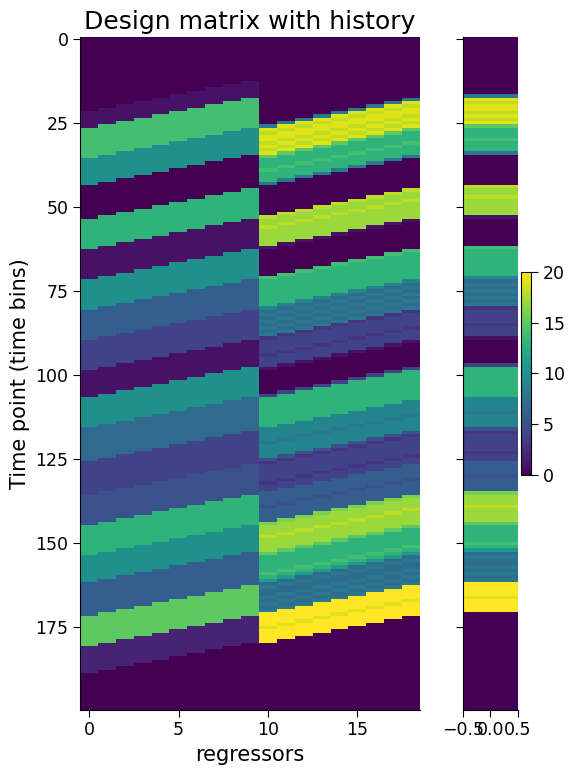
\[\begin{equation} \lambda = f(\theta x) = e^{\theta x}. \end{equation}\]Building a design matrix

Fitting GLM
You have a set of $Y={y_{i}}$ representing the number of spikes at time $t=i$ and corresponding stimulus and history features $X={x_{i}}$.
| To fit the GLM to spiking data, we want our parametrised distribution $P_{\theta}(y | x)≈P(y | x)$. This is achieved by finding $\theta$ which maximises our likelihood $P(Y | X, \theta)$. |
As each event is assumed to be conditionally independent, we can factorise the likelihood probability, which yields:
\[\begin{equation} P(Y|X,\theta) = \prod_{i}^{N} P(y_{i}|x_{i}, \theta) \end{equation}\]Taking the logarithm of the likelihood will speed up convergence and also reduces the complexity of the analytical solution:
\[\begin{equation} Log(P(Y|X,\theta)) = \sum_{i}^{N} y_{i}log(\lambda_{i}) -\lambda_{i} -log(y_{t}!) \end{equation}\]and in the recurrent linear-nonlinear Poisson model:
\[\begin{equation} \lambda_{i} = e^{x_{i}^{T}\theta} \end{equation}\]To find the maxima we take the derivative with respect to the $\theta$ which reduces to,
\[\begin{equation} \partial_{\theta} Log(P(Y|X,\theta)) = YX^{T} - X^{T}e^{X^{T}\theta}. \end{equation}\]Optimal kernels
After finding parameters that maximise the log-likelihood, we can define the best filters which then encode the stimulus input or neuron’s history.
Below are the optimal kernels for tonic spiking data. These filters are convolved along the time series.
Acknowledgements
This work replicates research by Weber, A. & Pillow, J. (2017).
Weber, A. I., & Pillow, J. W. (2017). Capturing the Dynamical Repertoire of Single Neurons with Generalized Linear Models. In Neural Computation (Vol. 29, Issue 12, pp. 3260–3289). MIT Press - Journals. https://doi.org/10.1162/neco_a_01021
Izhikevich, E. M. (2003). Simple model of spiking neurons. In IEEE Transactions on Neural Networks (Vol. 14, Issue 6, pp. 1569–1572). Institute of Electrical and Electronics Engineers (IEEE). https://doi.org/10.1109/tnn.2003.820440


