Understanding Dynamic Mode Decomposition: From Theory to Swimming
Published:
Introduction
Dynamic Mode Decomposition (DMD) is a data-driven technique for analysing complex dynamical systems. Originally developed for fluid dynamics, DMD has found applications across diverse fields including neuroscience, climate science, and biological locomotion. This method extracts coherent spatial-temporal patterns from high-dimensional time series data using autoregressive constraints.
The key insight behind DMD is that many complex systems can be approximated as linear transformations in an appropriate coordinate system. By identifying these coordinates and their associated temporal evolution, we can understand, predict, and control complex behaviors.
The DMD Algorithm
DMD seeks to find a linear operator $\bm{A}$ that best approximates the evolution of our system from one time step to the next. Given a sequence of snapshots arranged in matrices $\bm{X}$ and $\bm{Y}$, where $\bm{Y}$ contains snapshots that are one time step ahead of those in $\bm{X}$, we assume:
\[\bm{Y} = \bm{A}\bm{X}\]The challenge is that $\bm{A}$ is typically large and potentially ill-conditioned. DMD circumvents this by working in a reduced coordinate system.
Step-by-Step Algorithm
Step 1: Singular Value Decomposition
Decompose the data matrix $\bm{X}$ using SVD:
\[\bm{X} = \bm{U}\bm{\Sigma}\bm{V^{*}}\]where $\bm{U}$ contains the spatial modes, $\bm{\Sigma}$ contains the singular values, and $\bm{V}$ contains the temporal coefficients. The $*$ denotes complex conjugate transpose.
Step 2: Project onto Reduced Space
Compute the reduced-order representation of $\bm{A}$:
\[\tilde{\bm{A}} = \bm{U^{*}}\bm{A}\bm{U} = \bm{U^{*}}\bm{Y}\bm{V}\bm{\Sigma^{-1}}\]This projection dramatically reduces the computational burden while preserving the essential dynamics.
Step 3: Eigendecomposition
Find the eigenvalues $\lambda_i$ and eigenvectors $\bm{w}_i$ of the reduced matrix:
\[\bm{\tilde{A}}\bm{W} = \bm{W}\bm{\Lambda}\]where $\bm{\Lambda}$ is diagonal containing the eigenvalues, and $\bm{W}$ contains the eigenvectors.
Step 4: Reconstruct DMD Modes
Transform back to the original space to get the DMD modes:
\[\bm{\Phi} = \bm{Y}\bm{V}\bm{\Sigma^{-1}}\bm{W}\]These modes $\bm{\Phi}$ represent the spatial structures, while the eigenvalues $\bm{\Lambda}$ encode their temporal evolution.
Dynamics and Reconstruction
The reconstructed system evolves according to:
\[\bm{x}(t) = \bm{\Phi}\bm{\Lambda}^{t/\Delta t}\bm{\Phi^{\dagger}}\bm{x}(0)\]where $\bm{\Phi^{\dagger}}$ is the Moore-Penrose pseudoinverse and $\Delta t$ is the time step.
| Each eigenvalue $\lambda_i = | \lambda_i | e^{i\omega_i}$ encodes both growth/decay (through $ | \lambda_i | $) and oscillation frequency (through $\omega_i$). This makes DMD particularly powerful for identifying periodic behaviors and transient dynamics. |
Application: Zebrafish Tail Movement Analysis
Python implementation
import numpy as np
import numpy.linalg as linalg
def dmd(X, Y, truncate=None):
    if truncate == 0:
        # return empty vectors
        mu = np.array([], dtype='complex')
        Phi = np.zeros([X.shape[0], 0], dtype='complex')
    else:
        U2,Sig2,Vh2 = svd(X, False)
        r = len(Sig2) if truncate is None else truncate
        U = U2[:,:r]
        Sig = np.diag(Sig2)[:r,:r]
        V = Vh2.conj().T[:,:r]
        Atil = U.conj().T.dot(Y).dot(V).dot(linalg.inv(Sig)) # build A tilde
        mu,W = linalg.eig(Atil)
        Phi = Y.dot(V).dot(linalg.inv(Sig)).dot(W) # build DMD modes
    return mu, Phi
# process data
X = time_embedded[:, :-1]
Y = time_embedded[:, 1:]

# compute DMD modes
mu, Phi = dmd(X, Y, None)

# compute time evolution
b = np.dot(linalg.pinv(Phi), X[:,0])
Vand = np.vander(mu, np.max(X.shape), True)
Psi = (Vand.T * b).T
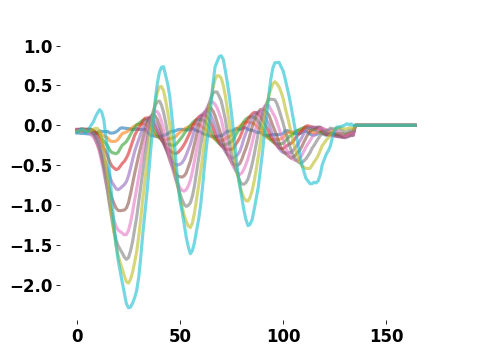
DMD Results
The evolution of the tail angle for a swim of a fish:
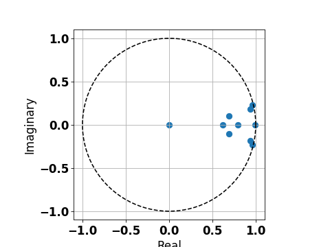
The eigen modes of the fitted DMD matrix
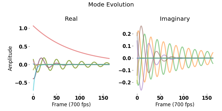
The different modes of tail behavior
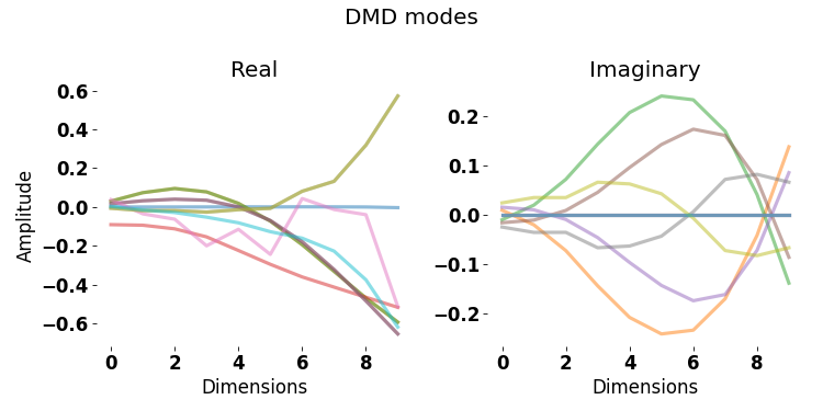
The evolution of these modes in reconstructing the original tail movement
Advantages and Limitations
Advantages:
- Model-free approach requiring no prior knowledge of governing equations
- Computationally efficient for high-dimensional data
- Provides both spatial and temporal information
- Well-suited for periodic and quasi-periodic systems
Limitations:
- Assumes underlying linear dynamics (in the DMD coordinate system)
- Sensitive to noise and measurement artifacts
- May struggle with strongly nonlinear or chaotic systems
- Requires careful selection of time delays and truncation parameters
References
- Schmid, P. J. (2010). Dynamic mode decomposition of numerical and experimental data. Journal of Fluid Mechanics, 656, 5-28.
- Kutz, J. N., Brunton, S. L., Brunton, B. W., & Proctor, J. L. (2016). Dynamic Mode Decomposition: Data-Driven Modeling of Complex Systems. SIAM.
- Tu, J. H., Rowley, C. W., Luchtenburg, D. M., Brunton, S. L., & Kutz, J. N. (2014). On dynamic mode decomposition: Theory and applications. Journal of Computational Dynamics, 1(2), 391-421.